Using ‘real’ data

#Install necessery Python packages

# Post spørring og få Pandas dataframe i retur
# benytter biblioteket pyjstat for JSON-stat

try:
    from pyjstat import pyjstat
    import requests
except:
    !pip install pyjstat
    from pyjstat import pyjstat
    !pip install requests
    import requests

# Import necessery Python packages
import pandas as pd # For data manipulation
import matplotlib.pyplot as plt # Import package for plotting

Loading the data

Here we follow step by step how the data was loaded. Feel free to skip this section!

Loading (installing) necessery Python packages:

1. Follow the link to find the data on CO2-emission from different sectors: https://www.ssb.no/statbank/table/13931/

2. Select the variables you are intersted in, see example below

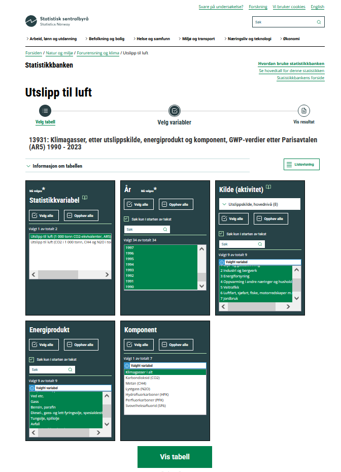
You can now vew this data as a table online. We can load it direcly by posting a SSB API query and using couple of Python commands!

3. Next, we copy the table URL and JASON query, and load the data (in json-stat2 format).

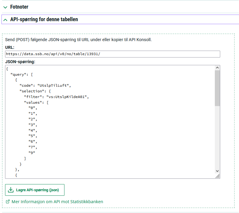
POST_URL = 'https://data.ssb.no/api/v0/no/table/13931/'
payload ={
  "query": [
    {
      "code": "UtslpTilLuft",
      "selection": {
        "filter": "vs:UtslpKildeA01",
        "values": [
          "0",
          "1",
          "2",
          "3",
          "4",
          "5",
          "6",
          "7",
          "9"
        ]
      }
    },
    {
      "code": "UtslpEnergivare",
      "selection": {
        "filter": "item",
        "values": [
          "VT0"
        ]
      }
    },
    {
      "code": "UtslpKomp",
      "selection": {
        "filter": "item",
        "values": [
          "A10"
        ]
      }
    },
    {
      "code": "ContentsCode",
      "selection": {
        "filter": "item",
        "values": [
          "UtslippCO2ekvival"
        ]
      }
    }
  ],
  "response": {
    "format": "json-stat2"
  }
}

resultat = requests.post(POST_URL, json = payload)

if resultat.status_code == 200:
    print('Data loaded successfully!')
else:
    print(f"Error: {resultat.status_code}")
    print(resultat.text)

Data loaded successfully!

If data loaded sucessfully, we need to tranform data to a format we can easily work with.

4. Turn JASON format resultat into a nice and tidy DataFrame df.

dataset = pyjstat.Dataset.read(resultat.text)
df = dataset.write('dataframe')
df.head() # print out the first 5 rows of the dataframe

	kilde (aktivitet)	energiprodukt	komponent	statistikkvariabel	år	value
0	Alle kilder	I alt	Klimagasser i alt	Utslipp til luft (1 000 tonn CO2-ekvivalenter,...	1990	51348
1	Alle kilder	I alt	Klimagasser i alt	Utslipp til luft (1 000 tonn CO2-ekvivalenter,...	1991	48987
2	Alle kilder	I alt	Klimagasser i alt	Utslipp til luft (1 000 tonn CO2-ekvivalenter,...	1992	47450
3	Alle kilder	I alt	Klimagasser i alt	Utslipp til luft (1 000 tonn CO2-ekvivalenter,...	1993	49379
4	Alle kilder	I alt	Klimagasser i alt	Utslipp til luft (1 000 tonn CO2-ekvivalenter,...	1994	51331

Exploring the loaded data

Let us explore and view the dataset. Type the following (one by one) in the code cells below

• df – to display the whole dataframe

• df.info() – to display information about the dataframe

• df.head() – to display the first 5 rows

• df.tail() – to display the last 5 rows

# Type any of the commands below to see the data in the dataframe

Some of the columns are redunant, and could be simply removed. Which ones?

#Let's count the number of occurrences of each unique value in another column of your DataFrame df.

That is right, we can simply drop ‘energiprodukt’, ‘komponent’, ‘statistikkvariabel’ columns:

df_cleaned = df.drop(columns=['energiprodukt', 'komponent', 'statistikkvariabel'])
df_cleaned

	kilde (aktivitet)	år	value
0	Alle kilder	1990	51348
1	Alle kilder	1991	48987
2	Alle kilder	1992	47450
3	Alle kilder	1993	49379
4	Alle kilder	1994	51331
...	...	...	...
301	Andre kilder	2019	2398
302	Andre kilder	2020	2341
303	Andre kilder	2021	2294
304	Andre kilder	2022	2242
305	Andre kilder	2023	2227

306 rows × 3 columns

We can also reshape our dataframe so that each entry tells you the emission value for a specific source and year.

# Pivot the table: year as index, kilder as columns, values filled in
data = df_cleaned.pivot(index='år', columns='kilde (aktivitet)', values='value')
data.title = "Utslipp til luft (1 000 tonn CO2-ekvivalenter)"
data.head()

kilde (aktivitet)	Alle kilder	Andre kilder	Energiforsyning	Industri og bergverk	Jordbruk	Luftfart, sjøfart, fiske, motorredskaper m.m.	Olje- og gassutvinning	Oppvarming i andre næringer og husholdninger	Veitrafikk
år
1990	51348	3084	341	19140	5050	5298	8254	2755	7426
1991	48987	2953	396	17620	4984	5109	8127	2490	7307
1992	47450	2924	390	15377	4956	5461	8728	2276	7338
1993	49379	2968	409	16325	4937	5664	9257	2308	7511
1994	51331	2999	466	17275	4944	5858	10053	2329	7408

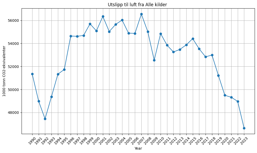
Let’s plot the emissions per year.

# plot value in the first column vs year

plt.figure(figsize=(10, 6))
#plt.plot(data.index, data['Alle kilder'], marker='o') # refer to the column by name
plt.plot(data.index, data.iloc[:, 0],  marker='o') # alternatively refer to the column by index


plt.title('Utslipp til luft fra Alle kilder ')
plt.xlabel('Year')
plt.ylabel( '1000 tonn CO2-ekvivalenter')
plt.grid(True)
plt.xticks(rotation=45)
plt.tight_layout()
plt.show()

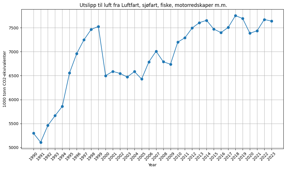
Modify the code below to plot emission from different sources per year.

# Plot
plt.figure(figsize=(10, 6))
#plt.plot(data.index, data['Alle kilder'], marker='o') # refer to the column by name
plt.plot(data.index, data.iloc[:, 5],  marker='o') # alternatively refer to the column by index

plt.title(' Utslipp til luft fra '+ data.columns[5])
plt.xlabel('Year')
plt.ylabel( '1000 tonn CO2-ekvivalenter')
plt.grid(True)
plt.xticks(rotation=45)
plt.tight_layout()
plt.show()